The beta-PERT Distribution

Overview of the beta-PERT distribution for modeling expert data

The beta-PERT distribution (from here on, I’ll refer to it as just the PERT distribution) is a useful tool for modeling expert data. When used in a Monte Carlo simulation, the PERT distribution can be used to identify risks in project and cost models based on the likelihood of meeting targets and goals across any number of project components.

As with any probability distribution, the usefulness of the PERT distribution is limited by the quality of the inputs: the better your expert estimates, the better results you can derive from a simulation.

This article describes the PERT distribution, how to use it, and its use within a Monte Carlo simulation. An additional discussion at the end describes the mathematical basis for the distribution, but an understanding of the math is not required to use the PERT distribution in your models.

Modeling Expert Data

In project or cost planning, you often receive estimates of expected time, cost, or other variables. To construct probability models (like Monte Carlo simulations), you will need a range of estimates – a minimum and maximum value, and if possible, a “most likely” value as well. These estimates are used to construct a probability distribution, and then a Monte Carlo simulation can be run based on samples from that distribution. (For a more general overview of Monte Carlo and probability simulations, see the whitepapers available on our library page).

When you have a range of estimates available, there are several different ways you can model the distribution to generate sample values. The three we discuss below are the uniform distribution, the triangular distribution, and the PERT distribution.

The Uniform Distribution

The uniform distribution is the simplest possible distribution for sampling a range of estimates. In this model, every value – from the minimum to the maximum – is equally likely.

Using the uniform distribution is useful in situations in which you have a minimum and maximum estimate available, but no other information. It’s easy to see that most real-world situations don’t fall into this model, and in many cases it’s possible to get an additional estimate of the expected, or most likely, value. If you can get a most likely estimate in addition to the minimum and maximum, you can use the additional information to create a more realistic probability model.

The Triangular Distribution

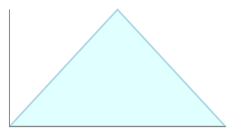
If you have a “most likely” estimate in addition to the minimum and maximum estimates, you can use this additional information to construct a probability distribution that favors the most likely value. The simplest distribution taking this into account is the triangular distribution – simply put, the distribution resembles a triangle with the most likely value (referred to as the mode) at the point of the triangle.

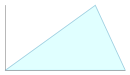
Examples of the triangular distribution: symmetrical and asymmetrical. The triangular distribution emphasizes the most likely result.

Unlike a uniform distribution, the triangular distribution emphasizes the most likely value, which should theoretically provide a better estimate of the probabilities of reaching other values. There is no requirement that the distribution be symmetrical about the mean; depending on the estimates you have for minimum, maximum, and most likely, the shape of the triangle may be skewed to the left (minimum) or right (maximum) values. In this way, the triangular distribution can model a variety of different circumstances.

However, by using a strict triangular shape about the mode, the triangular distribution may place too much emphasis on the most likely value, at the expense of the values to either side. The triangular distribution is useful in that it is easy to calculate and generate, but it is limited in its ability to model real-world estimates.

The PERT Distribution

The PERT distribution also uses the most likely value, but it is designed to generate a distribution that more closely resembles realistic probability distribution. Depending on the values provided, the PERT distribution can provide a close fit to the normal or lognormal distributions.

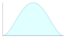
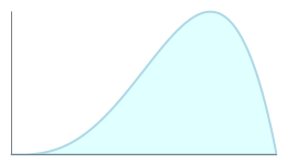
Like the triangular distribution, the PERT distribution emphasizes the “most likely” value over the minimum and maximum estimates. However, unlike the triangular distribution the PERT distribution constructs a smooth curve which places progressively more emphasis on values around (near) the most likely value, in favor of values around the edges. In practice, this means that we “trust” the estimate for the most likely value, and we believe that even if it is not exactly accurate (as estimates seldom are), we have an expectation that the resulting value will be close to that estimate.

Examples of the PERT distribution: compare the smooth curves to the triangular distribution, above. Values near the peak are more likely than values near the edges.

Assuming that many real-world phenomena are normally distributed, the appeal of the PERT distribution is that it produces a curve similar to the normal curve in shape, without knowing the precise parameters of the related normal curve.

Using the PERT Distribution in Excel with the RiskAMP Add-in

The RiskAMP function PERTValue samples from the beta-PERT distribution. Here’s an example of the PERTValue function, compared to the Triangular distribution (if you change the values, click the “play” button to run a simulation and update the charts):

The simple case of the PERT distribution takes a minimum, maximum, and most likely value. The RiskAMP function PERTValue uses these inputs to generate a random sample from the distribution:

=PERTValue( Minimum, MostLikely, Maximum )

The scale, or λ (lambda) parameter, can also be used to modify the distribution:

=PERTValue( Minimum, MostLikely, Maximum, Lambda )

But use of the scale parameter is optional. If omitted, the default scale value is 4, which produces a curve that reasonably approximates the normal distribution.

A second function, PERTValue.P, uses the same distribution but takes as parameters the 10th and 90th percentile values. You would ordinarily use this function if your estimates exclude the tail (or most unlikely) probabilities.

The sample spreadsheets that are installed with the RiskAMP Add-in include a project/task model using the PERT distribution. That model demonstrates how to use the PERTValue function and how to display and chart probabilities based on a PERT distribution.

The Mathematical Model

The PERT distribution is a special case of the beta distribution that takes three parameters: a minimum, maximum, and most likely (mode). Unlike the triangular distribution, the PERT distribution uses these parameters to create a smooth curve that fits well to the normal or lognormal distributions.

The beta distribution is characterized by the density function

$$ f(x) = \begin{cases} \frac{x^{v-1} \left ( 1-x \right )^{w-1}}{B(v,w)} & 0 \le x \le 1 \\ 0 & \text{otherwise} \end{cases} $$

and the distribution function

$$ F(x) = \begin{cases} \frac{ B_{x}(v, w) }{ B(v, w) } & 0 \le x \le 1 \\ 0 & \text{otherwise} \end{cases} $$

Sampling from the beta distribution requires minimum and maximum values (scale) and two shape parameters, v and w.

The PERT distribution uses the mode or most likely parameter to generate the shape parameters v and w. An additional scale parameter λ scales the height of the distribution; the default value for this parameter is 4.

In the PERT distribution, the mean μ is calculated

$$ \mu = \frac{ x_{min} + x_{max} + \lambda x_{mode} }{(\lambda + 2)} $$

and used to calculate the v and w shape parameters

$$ v = \frac{ ( \mu - x_{min} )(2 x_{mode}-x_{min}-x_{max}) }{(x_{mode}-\mu)(x_{max}-x_{min})} $$

$$ w = \frac{v(x_{max}-\mu)}{(\mu-x_{min})} $$

which are used, with the minimum and maximum scale parameters, to sample the beta distribution.

The beta-PERT Distribution in R

Here is an implementation of the beta-PERT distribution in R, using the native beta function:

rpert <- function( n, x.min, x.max, x.mode, lambda = 4 ){

    if( x.min > x.max || x.mode > x.max || x.mode < x.min ) stop( "invalid parameters" );

    x.range <- x.max - x.min;
    if( x.range == 0 ) return( rep( x.min, n ));

    mu <- ( x.min + x.max + lambda * x.mode ) / ( lambda + 2 );

    # special case if mu == mode
    if( mu == x.mode ){
        v <- ( lambda / 2 ) + 1
    }
    else {
        v <- (( mu - x.min ) * ( 2 * x.mode - x.min - x.max )) /
            (( x.mode - mu ) * ( x.max - x.min ));
    }

    w <- ( v * ( x.max - mu )) / ( mu - x.min );
    return ( rbeta( n, v, w ) * x.range + x.min );
}

For more information and a more detailed analysis, see (e.g.) Risk Analysis – A Quantitative Guide, by David Vose (John Wiley & Sons, 2000). [Amazon]